Tools

In this tab, you will find various auxiliary functions that are not part of the main modules. These include a tool for calculating alternative shadows (different from those generated during placement), a function for inserting reports into drawings, a parts list generation feature, and a surface analysis tool.

Shadow

Visualize Shadows on Modules

Here, you can display the direct shadows cast on the modules and interactively simulate how they change using the sliders.

Date / Time
Enter a specific date for the shadow calculations. Use the single arrow button to select a date from the calendar, or adjust individual components of the date using the up/down buttons.

DST (Daylight Saving Time)
Enable or disable daylight saving time to adjust sunrise and sunset times accordingly. This will also refresh the displayed shadows.

Sunrise / Sunset
View the automatically calculated sunrise and sunset times for the selected date. These calculations account for the geographical position and DST setting.

Calculation Interval
Define the time interval for shadow calculations throughout the day.

Calculate Each
Choose whether results are displayed per array or per module. Note that displaying results per module increases computation time significantly.

Calculation Mode
Select the desired calculation mode:

• Fast: Considers shadows cast only by arrays in the immediately preceding row.
• Exact: Includes shading influences from all arrays, even distant ones, for a more detailed result.

Change Day
Modify the date, which will automatically update the displayed shadow calculations.

Change Time
Adjust the time, and the displayed shadows will refresh accordingly.

On/Off
Toggle the display of calculated shadows on or off.

View
Choose the type of results to display: the shadows on the modules, the percentage of shading, or both.

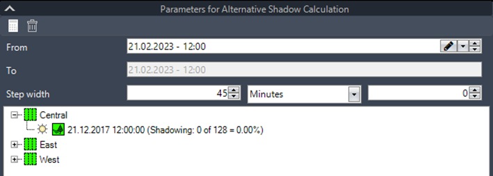
Parameters for alternative Shadow Calculation

Here, you can perform an additional shadow calculation for all arrays within one or more fields. This calculation generates and displays a new shadow, similar to the one used for determining the row distance during placement.

(Surface) Grading Function

The grading function enables modification of the surface by cutting specific areas and optionally filling others, based on the distances to the racks of an existing PV layout. This process creates a new, graded surface beneath the selected arrays, eliminating the need to lift arrays to achieve a specific clearance.

Requirements for grading

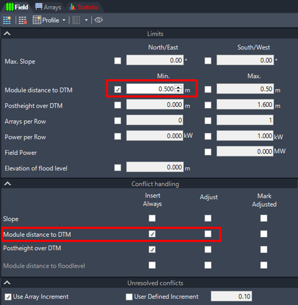
To ensure the placement on the new surface matches the original layout, a PV layout must be created without any height adjustments to arrays that have a module-DTM clearance conflict.

In the placement options, configure the module distance to the DTM and select the “Insert Always” option while leaving “Adjust” unchecked. This ensures that the original layout remains unchanged, even in cases of clearance conflicts.

For example, if the array height is set to 0.8 m in the array definition, and the module-DTM distance is configured to 0.50 m, the layout will maintain these specifications without adjustments.

Create Grading Zone

The grading function, found under the Tools menu, requires the user to select a group of arrays. These arrays must be directly adjacent to each other. If the arrays are farther apart, you will need to perform multiple grading operations sequentially.

Each group of arrays forms a separate grading zone, similar to islands, which are then integrated with the original surface. In the example below, a pair of arrays is shown, with the first array selected for grading.

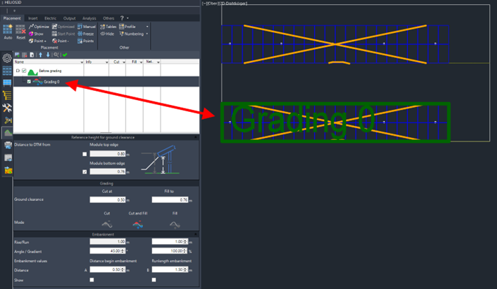
For eachgrading zone you can set the below options for the graded surface.

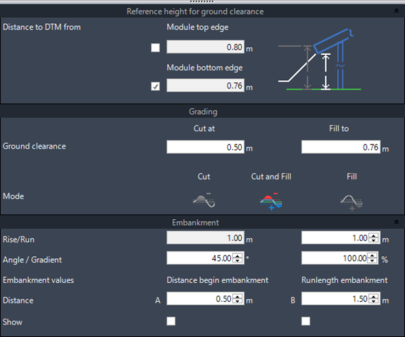
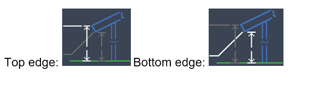
Distance to DTM From
The cut and fill distances are measured from either the top or bottom edge of the module. These values are determined by the array definition properties and cannot be modified here.

The preview on the right visually indicates the selected edge, highlighted in white.

Ground Clearance
Set the distance for cut and fill operations. Areas closer than the specified distance will be cut, while areas further away will be filled.

Mode
You can choose from the following options:

• Cut Only
• Fill Only
• Cut and Fill (both operations performed simultaneously)

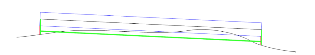
Embankment
An embankment is created to smoothly transition the grading zones with the original surface. The Rise is fixed at 1 meter, and the Run can be adjusted to calculate the Angle and Gradient. When either the Angle or Gradient is changed, the other value, along with the Run, is automatically recalculated.

Distance to Begin Embankment
Set the starting distance from the arrays to ensure the embankment edge doesn’t align directly with the array edges.

Run Length of Embankment
Limits the maximum length of the embankment to prevent overly long transitions, which can occur if the angle is too shallow.

Show
Displays temporary polylines that represent the set distances for the embankment, providing a visual reference for the grading layout.

Create Grading Surface

The grading surface is generated based on the selected zones, integrating the cut and fill operations to create a smooth, adjusted surface beneath the arrays.

The generated surface is a standard TIN (Triangulated Irregular Network) surface, which is displayed in both the Autodesk Civil 3D Toolspace and the placement list of the Helios 3D palette.

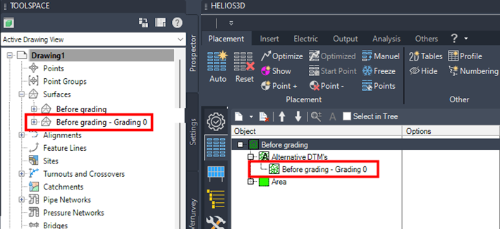
The graded surface can be set as the Helios3D surface, which will reset the existing PV layout. To do this, right-click on the graded surface in the context menu and select the „To Helios3D surface“ command.

Now placements use the graded surface and the original is displayed as alternative DTM.

Grading reference edges for tracker arrays

For tracker layouts created in earlier program versions up to 2024, the placement must be renewed to ensure that the orientation of each tracker is maintained relative to the graded terrain.

For detailed information on how trackers are rotated to align with the ground, please refer to section „Insertion/rotation of a tracker array to the surface“.

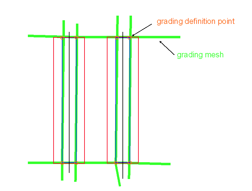
The grading surface (represented in green) is created using the two reference points at the beginning and end of the tracker, which are established during the tracker insertion. A planar surface is then generated between the rows, connecting these tracker reference points. The distance for cut and fill can be set individually based on the module’s bottom edges.

The grading reference points correspond to 3D coordinates located beneath the lowest module points at the start and end of the tracker. This ensures that the tracker placement on the graded terrain remains consistent with the original layout.

Reports as background pictures

Here, you can generate reports and insert them into the drawing. Various pre-defined reports are available in the Helios 3D installation directory, located under the path .\Reports\System.

In the future, we plan to offer the option for you to add custom reports to the .\Reports\User folder. These reports can be created using the reporting tool located in the Helios 3D Bin folder.

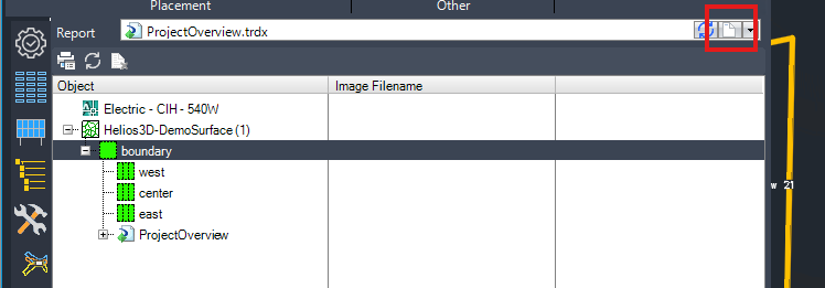
In the „Report“ line, you can select a report from the refreshable list. Alternatively, you can open the report designer by clicking the corresponding button.

Insert Selected Report

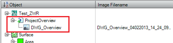
Clicking the „Generate Report“ button creates the report selected in the dropdown menu, using the filter settings defined by the element selection in the list below. Available filters include the complete drawing (e.g., „Test_ZWR“ in the figure), a specific area, or a field.

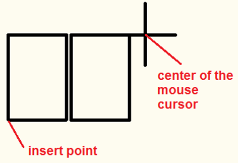
Upon pressing the button, you will be prompted to enter a name for the report. After naming it, you can insert the report into the drawing by selecting a location with your mouse.

• The first click defines the insertion point for the first page of the report.
• Subsequent pages are displayed schematically as frames, as shown in the next figure.
• You can adjust the page size and arrangement (row-wise, column-wise, or in a block of multiple rows and columns) by moving your mouse.

A final left-click confirms and inserts the pages into the drawing.

Refresh Selected Report

The Refresh button updates the report selected in the list. To refresh, ensure that the entry for the report base or one of its images/pages (child nodes) is selected in the list. These selectable nodes are highlighted in the following figure.

Delete Selected Report

The Delete button removes the report selected in the list. To delete, ensure that the entry for the report base or one of its images/pages (child nodes) is selected in the list. These nodes are indicated in the previous figure.

Analysis

Here, you can add and manage terrain analysis results, enabling a detailed evaluation of the surface characteristics and their impact on the project layout.

Add Terrain Analysis

This function allows you to generate a terrain analysis for a web browser in the upcoming dialog and then transfer the result back to the CAD system. If a browser export has not been initiated yet, this function can optionally start the export process as well.

Delete Terrain Analysis

This function deletes the result entry and its associated contents for the selected terrain analysis.

Freeze Results

This function freezes the layers of any analysis displayed in the list below, preventing further changes or updates to those layers while keeping them visible.

When a terrain analysis is added, the calculation occurs in the web browser view. If no active connection to a running browser export is found, the system will initiate the browser export process. Once this is done, the following dialog will appear.

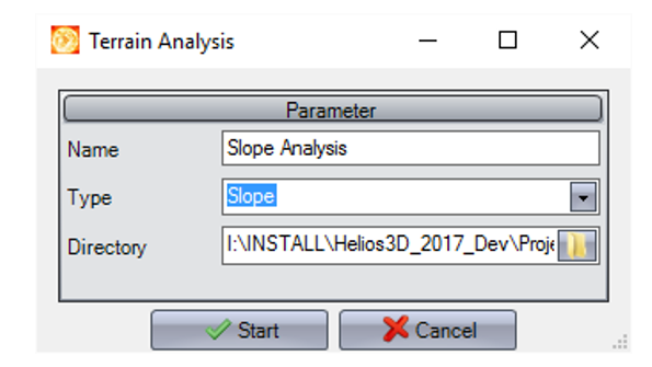
Name
Enter a name for the analysis. The result will be displayed under this name in the HELIOS 3D palette.

Type
Select the type of analysis you want to start by clicking . The result will then be transferred to and displayed within the application.

Directory
Choose the directory where the result file will be saved. By default, the result image will be saved to the project folder.