Analysis
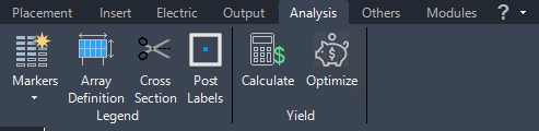
Command Group Legend
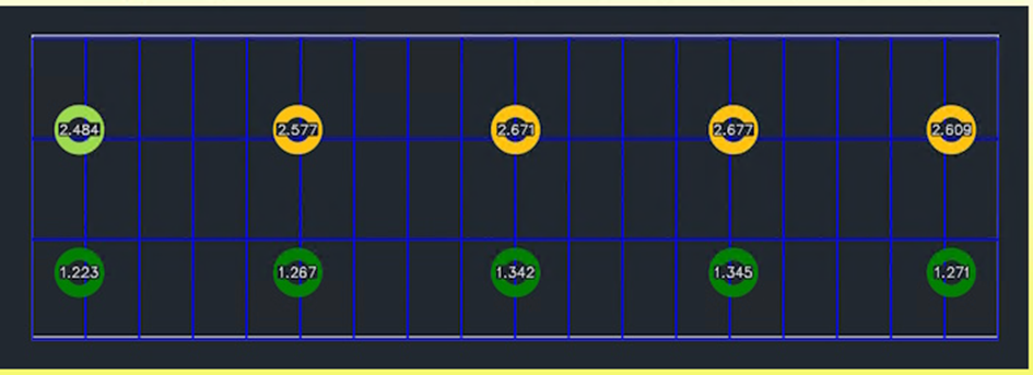
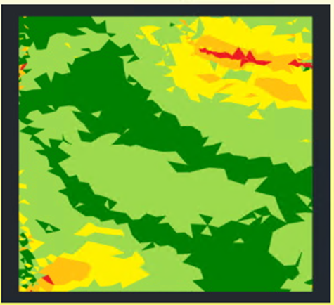
Marker Schemes
Functions for different marker schemes for arrays, posts, modules and surfaces. For each type, intervals can get defined with separate colors for temporary hatches or circles. The snapshot command will change displayed temporary hatches into standard AutoCAD objects.


Hide Markers

Hides all displayed markers.
Create snapshot

Creates a snapshot from the displayed temporary hatches belonging to marker schemes. These get inserted as AutoCAD hatches, which are selectable and printable.
Delete snapshots

Deletes all objects on the layer „H3D_Snaphost“.
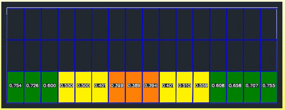
Create post markers to filter report
Opens the dialog for creating a post marker scheme for the selected fields. On printing a post report, you can choose to just include such marked posts.
Delete post markers for reports
Deletes post markers from the drawing.
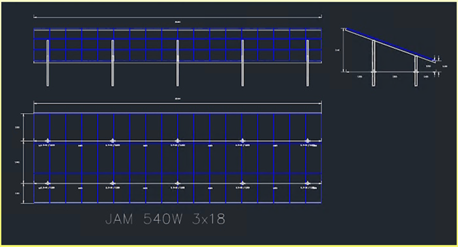
Insert Array Legend
Calls the dialog for creating an array legend, which can show the top, front and side view for the array definition. The legend includes measurements of geometry. This function uses the dimensioning style „H3D_AL“ for Array Legends.
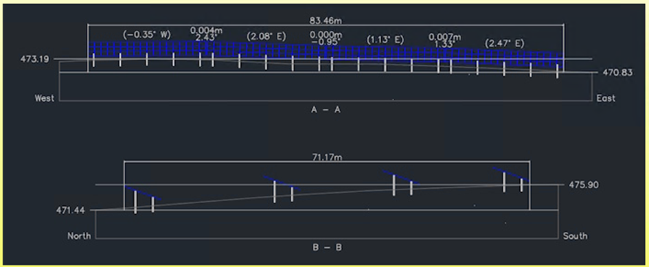
Create Cross Section View
You can create a cross section along a row or perpendicular through rows. This function uses the dimensioning style „H3D_CS“ for Cross Section views.
Command Group Yield
Run Yield Assessment

Opens the dialog yield assessment for the current layout, which contains the parameters and device values for the calculation of total yield over a year. This function allows us to compare different layouts and find the yield-oriented optimum.
Run Module Angle Optimization

Opens the dialog for optimizing the module inclination angle and the orientation angle of the modules / array rows. For that, the effects of different module inclination angles and array orientations to the resulting power get checked on a flat surface. The resulting report shows the ideal orientation of the modules under simplified conditions.