
Placement
This section contains all commands for placing arrays and is activated automatically whenever the user opens the „Placement“ module.
The Placement ribbon is used during the layout phase of a PV project. It contains the main commands for generating, adjusting, optimizing, resetting and documenting the array placement inside defined fields. In Helios 3D, these commands affect the physical arrangement of PV tables, rows, start points, conflict markers and placement-related drawing objects.
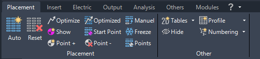
Command Group Placement
Before using the placement commands, make sure that the relevant project, drawing and fields are available and that an array definition has been selected or configured. For automatic placement, the field geometry, exclusion zones, terrain data and placement settings should be checked first. If the placement result does not match the expected layout, review the field boundary, exclusion zones, row distance settings, slope limits and array definition before repeating the placement.
Automatic Placement

Automatically locates a starting point for the placement of the first row. The initial array is positioned at the southernmost edge of the field, with each row placed from left to right. This direction can be reversed by selecting the “Place Right-Aligned” option in the placement settings.
Use Automatic Placement when a complete field should be filled according to the current placement settings. The result depends on the selected field, the active array definition, the allowed placement area and the configured placement rules. If arrays are not placed as expected, check whether the field is too small, blocked by exclusion zones, affected by terrain restrictions or influenced by the selected placement direction.
Reset Placement

Resets the array placement for all selected fields.
Use Reset Placement when an existing placement result should be removed from the selected fields before recalculating or manually rebuilding the layout.
This command should be used carefully, because it changes the current placement state of the selected fields.
Place and optimize
This option initiates an automatic placement process, displaying a dialog for setting the optimization increment and estimating the calculation time. Alternative layouts are generated by shifting the start row according to the specified increment.
The function stops when the new start point aligns with the second row’s start point from the original calculation. The layout with the maximum power output is then displayed as the result.
The optimization compares alternative start positions and can therefore take longer than a standard automatic placement. A smaller optimization increment may create more layout variants and can increase calculation time. Use this function when the starting position of the first row may influence the usable number of arrays or the total installed power.
Place using the start point from last optimization
Initiates placement using the last saved starting point generated by the optimized placement function.
Insert Arrays Manually
Opens a dialog for manually adding a new array row or inserting arrays into an existing table row. This feature allows for a fully manual table layout, for example, by adjusting the module inclination angle, without altering the row distances.
Manual insertion is useful for correcting individual gaps, adding specific PV tables or creating a layout that intentionally differs from the automatic placement result. The command can be used to add a new row or to insert arrays into an existing row. Manual changes should be checked against the same technical constraints as automatic placement, such as field borders, exclusion zones, terrain clearance, slope limits and available row gaps.
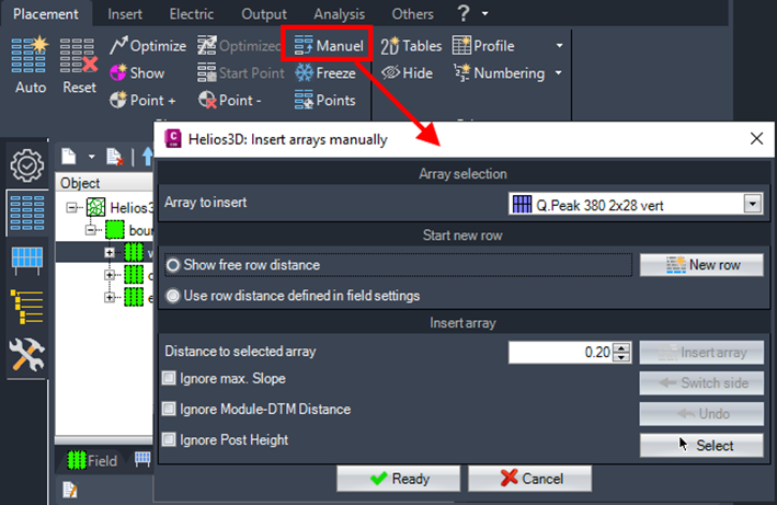
To add a new row to a table, you can either position it freely with your mouse or use the specified placement settings.
To insert a table into an existing row, follow these steps:
Reference Table: Begin by selecting the reference table.
Placement Conflicts and Preview Colors: The preview rectangle for the selected array definition, chosen from the list of requirement types, will display a color corresponding to any placement conflict that prevented insertion in regular placement mode:
- Cyan: Side slope exceeded
- Orange: Insufficient distance to module-DTM
- Purple: Post length limitations
- Red: The array does not fit within the available gap
The preview color indicates why the current insertion position may not be valid in regular placement mode. If a conflict is ignored for the current insertion, the layout should be checked manually afterwards. Ignoring a conflict may be acceptable for a specific design decision, but the technical consequence should be validated before using the result for further planning or evaluation.
Conflict Resolution Options: You can adjust the distance to the selected array, ignore conflicts for the current insertion, or alter the gap by modifying the field border or exclusion zone. Once any conflict is resolved or ignored, the option to proceed becomes available.

You may also choose to move the insertion to the opposite side of the selected table or reset all changes.


Finalizing Changes: Only selecting the „Apply Changes“ option will confirm and finalize all adjustments.
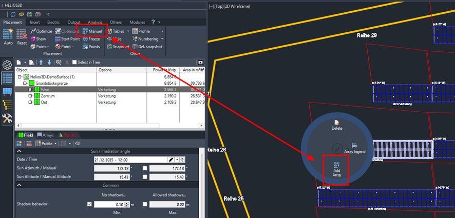
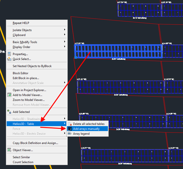
The command for adding a PV table to an existing design has been added to the radial menu and the context menu of existing table insertions.
The below figures show the two commands, which have the advantage that the calling table insertion is already set as current reference table. This saves the extra clicks for choosing the reference table in the upcoming dialogue.
Show Start Point
You can view the position of the first array row by hovering over the insertion point in the drawing with your mouse.
Place with shown start point

The last start point used by the „Show Start Point“ function will be applied for the placement.
Freeze Placement
Freezing the current placement will create a manual row start point for any table row.
After that the current layout can be replaced with a different module inclination, without any change to the row distances.
Freeze Placement is helpful when the row positions should remain fixed while other array-related parameters are changed. This can be useful for comparing design variants, for example when the module inclination is adjusted but the existing row spacing must be preserved. After freezing, verify that the new array configuration still fits the field and does not create new placement conflicts.
Define row start points manually (only for manual placement)
Add start points for each row of arrays with your mouse. Each point insertion will start a new row, ignore all row distance or shade settings.
There is a separate placement command to use these points, and the automatic placement will ask whether start points should be used, when detected.
Manual row start points override the normal automatic row spacing logic for the affected placement process. Use this option only when the row positions are intentionally controlled by the user. Because row distance and shade settings are ignored for these start points, the resulting layout should be checked for shading, spacing, collision and terrain-related restrictions.
Delete all rows start points
Deletes all row start points registered to the selected fields.
Place with Defined Start Points
Place arrays based on manually defined start points for the selected fields (one row per start point). If any disturbance occurs during the placement of a row, the process will be immediately aborted, but only for that specific row. In such cases, another start point definition must be provided before attempting the manual placement again.
If placement with defined start points fails for one row, review the corresponding start point, the available field width, nearby exclusion zones and the selected array definition. A new or adjusted start point may be required before the row can be placed successfully.
Command Group Other

Create 2D Projections
Generates a rectangular 2D polylines for any array, representing the 2D projection. Several variants for the module area only, each module and the substructure are available. The table front edge is used as base line.
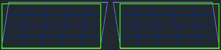
Placement options can be saved as a profile in the database, allowing them to be loaded into any drawing, regardless of the project.
Placement profiles are useful when the same placement settings should be reused across drawings or projects. Loading a profile applies the saved settings to the current drawing context. Before overwriting, renaming or deleting a profile, make sure that the profile is not still needed as a standard setting for other layouts or users.
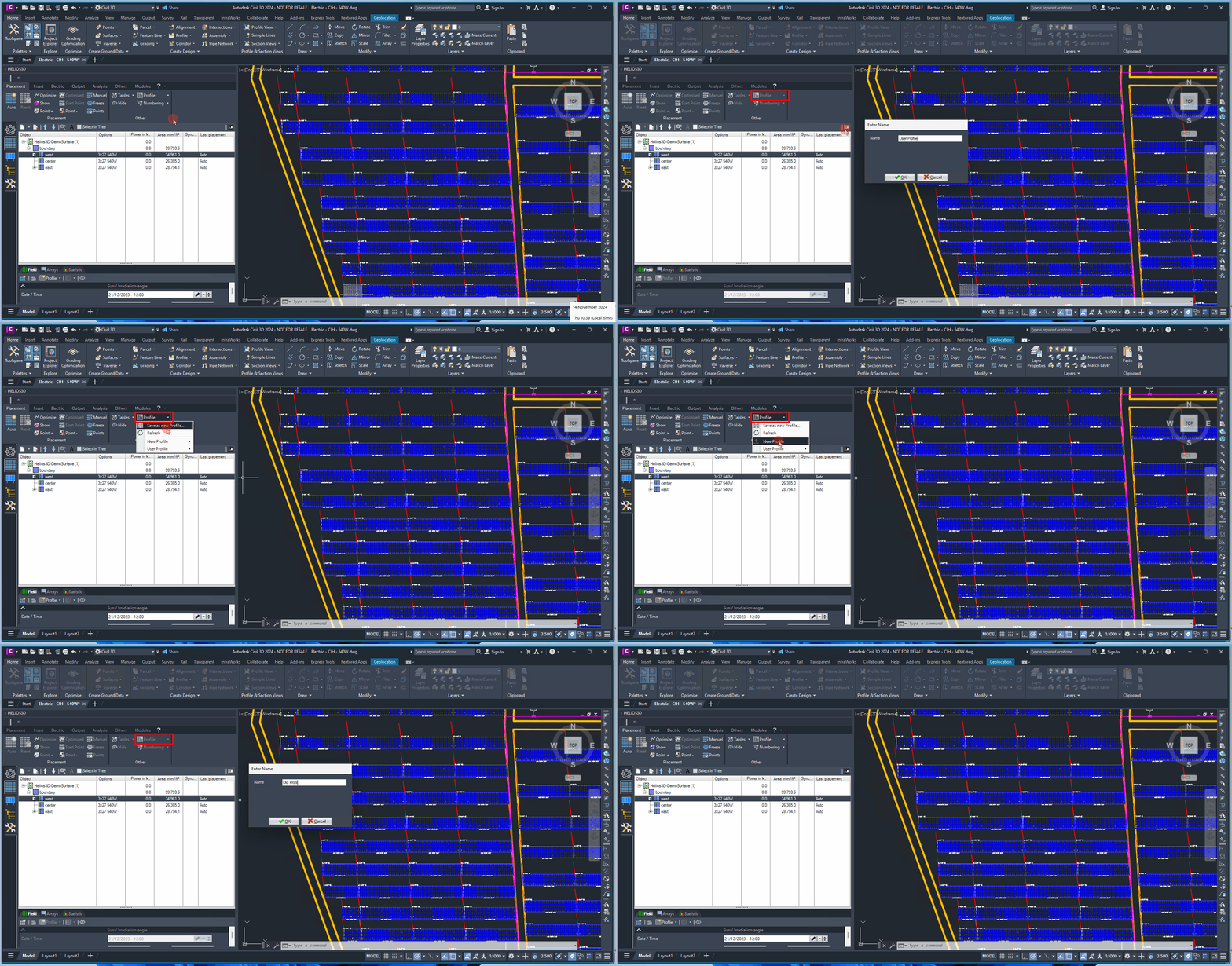
Save as new Profile
Opens the menu to save the current settings as a profile. From here, you can save the placement settings as a new profile.
Refresh
Updates the data from the current profile.
Load
Opens the menu to select a saved profile. Upon selection, all associated settings are loaded.
Overwrite
From there, you can overwrite the existing placement settings profile.
Rename
Renames an existing profile.
Delete
Deletes an existing profile.
Hides all Conflict Markers from Placement

During placement all positions with array / DGM collisions or increasing maximum slope were marked with colored rectangles.
With this command you can delete all those rectangles.
This command removes the visual conflict markers from the drawing. It does not automatically solve the underlying placement conflict. If the same placement is calculated again without changing the relevant settings or geometry, similar conflict markers may appear again.
Row and Array Numbering

Contains functions for creating or applying an individual numbering scheme to the selected fields.
Row and array numbering helps identify PV tables in drawings, reports, coordination workflows and later project documentation. A consistent numbering scheme is especially important when layout data is used for electrical planning, installation coordination, quantity checks or external communication.
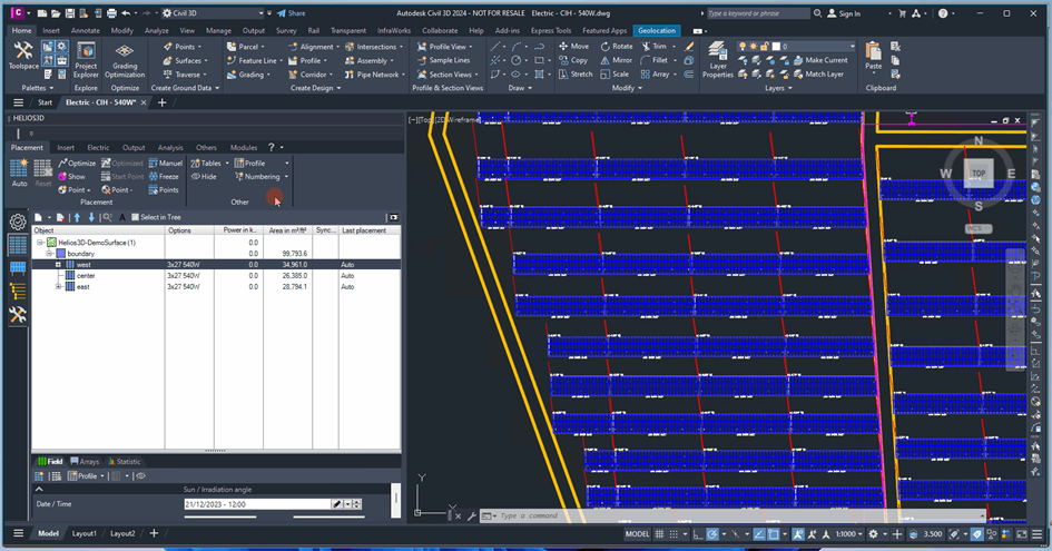
Row and Array Numbering Dialog
Opens the dialog for creating and applying a numbering scheme for array rows and arrays of the selected fields.
Refresh Row and Array Numbering
This will renumber all fields selected in the tree while each field uses its own saved settings.
Numbering Direction
Allows you to change the numbering according to the directions shown by the active arrow button.
Rows
- Row text
Activate to set a custom text for an individual row. - Starting number
Set the starting number for the first row of the field. - Numbering per
The row numbering can be configured either field-wise (where each field starts with row number 1) or sequentially across fields, with numbers continuing based on the sort order in the list.
Arrays
- Array prefix
Activate if you want to add a prefix (custom text) before the table number. - Row prefix / Delimiter
Activate if you want to set a prefix, such as a shortcut for the field. In the second field, you can choose a delimiter, either a dot or a comma. - Starting number
Set the starting number for the first array in the selection. - Numbering Mode
The numbering will begin with the specified starting number for each row or field, or it can continue sequentially across all fields according to the order in the list below.
Numbering Rows, PV Tables and Posts
The numbering function is used to assign and update identification texts for rows, PV tables and posts in a Helios 3D drawing. The revised dialog separates the three object types into the individual tabs Rows, Tables and Posts.
Use this function after the placement has been completed and the affected fields contain the final rows, tables and posts. If the placement is changed later, the numbering may need to be repeated.
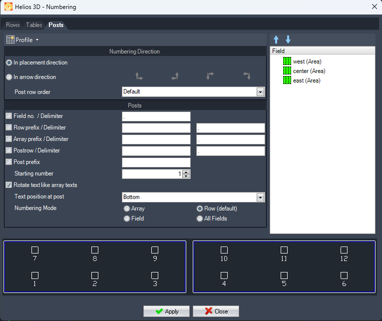
Dialog Structure and Workflow
The numbering dialog contains separate tabs for rows, PV tables and posts. Each tab provides the settings required for the selected object type.
The active tab determines which numbering operation is executed when Apply is selected. For example, if the Posts tab is active, only the post numbering is applied.
The numbering result is previewed at the bottom of the dialog before it is inserted into the drawing. Review this preview to verify the selected direction, order, prefixes, delimiters and starting number.
The revised dialog can override project settings that would otherwise prevent certain labeling texts from being inserted. This makes it possible to create the selected numbering directly from the dialog even if the corresponding project-level text setting is disabled.
Image position: Insert the screenshot of the numbering dialog from page 2 of the PDF here.
Image caption: Numbering dialog with separate tabs for rows, PV tables and posts
Profiles
Each tab contains its own profile selection. A profile stores the numbering settings of the active tab so that the same configuration can be reused in other projects.
Because the profiles are managed separately for rows, tables and posts, selecting or changing a profile on one tab does not define the settings of the other tabs.
Use separate profile names when different numbering conventions are required for specific customers, projects or output formats.
Numbering Direction
The numbering direction determines the order in which the selected objects receive their numbers.
The following options are available:
In placement direction: The objects are numbered according to the direction in which the PV tables were placed.In arrow direction: The numbering follows the manually selected arrow direction.
When arrow-based numbering is selected, use the direction buttons displayed in the dialog to define the required starting side and counting direction. Check the preview before applying the numbering.
Posts
The Posts tab controls how post numbers and post labels are generated. It provides settings for the counting order, prefixes, delimiters, starting number, text orientation, text position and numbering scope.
The final post label can be assembled from several optional components. Only enabled components are included.
Post Row Order
Post row order defines the sequence in which the post rows inside the selected tables are processed. The result can also depend on the selected numbering mode.
The following options are available:
Default: Maintains the numbering sequence in the same direction for every post row.Serpentine: Reverses the numbering direction for every second post row. This creates an alternating back-and-forth numbering sequence.Reverse post rows: Reverses the internal order of the post rows within a table. This option is relevant when posts are numbered per field.
Use the preview to check whether the selected post row order corresponds to the required installation, surveying or documentation sequence.
Number Components
The post number can contain field, row, table and post-row information. These components are added as prefixes before the actual post number.
Each component is optional. Enable only the elements that are required for the intended numbering convention.
Field No. / Delimiter
Enable Field no. to add the field identifier as a prefix to the post number.
Enter a delimiter to separate the field identifier from the following part of the post label.
For example, a field identifier F01, a delimiter - and a post number 15 can produce:
F01-15
Row Prefix / Delimiter
Enable Row prefix to add a row-related identifier before the post number.
The delimiter separates the row identifier from the following part of the label. Use this option when the post number must indicate the row to which the post belongs.
Table Prefix / Delimiter
Enable Table prefix to include the identifier of the PV table in the post label.
The specified delimiter is inserted between the table identifier and the following numbering component.
Use this option when post numbers must remain traceable to individual PV tables.
Post Row Prefix / Delimiter
Enable Post row prefix to include an identifier for the post row within the PV table.
The delimiter separates the post-row identifier from the following part of the label. This option is useful for tables containing more than one row of posts.
Post Prefix
Enable Post prefix to insert a fixed text before the numerical part of the post number.
For example, the prefix P and the number 15 can produce:
P15
Unlike the field, row, table and post-row options, the post prefix does not have a separate delimiter field. If a separator is required, include it directly in the prefix.
Starting NumberStarting number defines the first numerical value used when the selected posts are renumbered.
The way the numbering continues or restarts depends on the selected numbering mode. For example, a starting number of 1 restarts at 1 for each new table when the Array mode is selected.
Rotate Text Like Array Texts
Enable Rotate text like array texts to align the post label with the orientation of the
corresponding PV table.
If this option is disabled, the text uses a fixed drawing orientation with a north-up alignment.
Enable this option when post labels should visually follow rotated or differently oriented PV tables.
Text Position at PostText position at post defines where the generated label is inserted in relation to the post.
Select the required position from the available list. Check the preview and the resulting drawing to make sure that the text does not overlap the post geometry, dimensions or other annotations.
Numbering Mode
The numbering mode defines the scope within which post numbers are counted and the point at which the starting number is reused.
ArrayArray counts the posts within an individual PV table. When the next table is processed, numbering restarts at the defined starting number.
Use this mode when every PV table requires its own independent post-number sequence.
Table RowTable Row is the default numbering mode.
It counts the posts within a table row and restarts the numbering for each new table row.
Use this mode when each row of PV tables requires an independent post-number sequence.
FieldField counts the posts continuously within one field. The numbering restarts at the defined starting number when the next field is processed.
Use this mode when every field requires its own complete and independent sequence.
All FieldsAll Fields counts the posts continuously across all selected fields.
The numbering does not restart when the next field is processed. The order of the fields in the field list therefore affects the resulting numbers.
Use this mode when all selected fields must share one continuous post-number sequence.
Field List
The field list shows the fields included in the current numbering operation.
Use the arrow buttons beside the list to change the processing order. This order is particularly important when All Fields is selected because the numbering continues from one field to the next.
Before applying the numbering, verify that:
- all required fields are listed;
- no unintended field is included;
- the fields are arranged in the required counting order;
- the preview corresponds to the expected result.
Applying the Numbering
After configuring the active tab, review the preview at the bottom of the dialog.
Select Apply to execute the numbering for the currently active tab. The settings of the other tabs are not applied automatically.
If rows, tables and posts must all be numbered, configure and apply each tab separately.
Close the dialog only after all required numbering operations have been completed.
Important Considerations
Numbering should be performed after the placement structure is stable. Changes to fields, rows, PV tables or posts can make existing labels outdated.
Before applying a new numbering scheme, check whether existing numbering texts should be replaced or removed to avoid duplicate labels.
When using prefixes and delimiters, make sure that the resulting labels remain unique and readable. Similar identifiers for fields, rows, tables or post rows can otherwise produce ambiguous post numbers.
When All Fields is selected, the field order directly affects the continuous numbering sequence. Always verify the field list before selecting Apply.
The preview represents the configured numbering scheme. After execution, also inspect the labels in the drawing, especially where PV tables are rotated or where posts, dimensions and other annotations are positioned close together.
Create snapshot
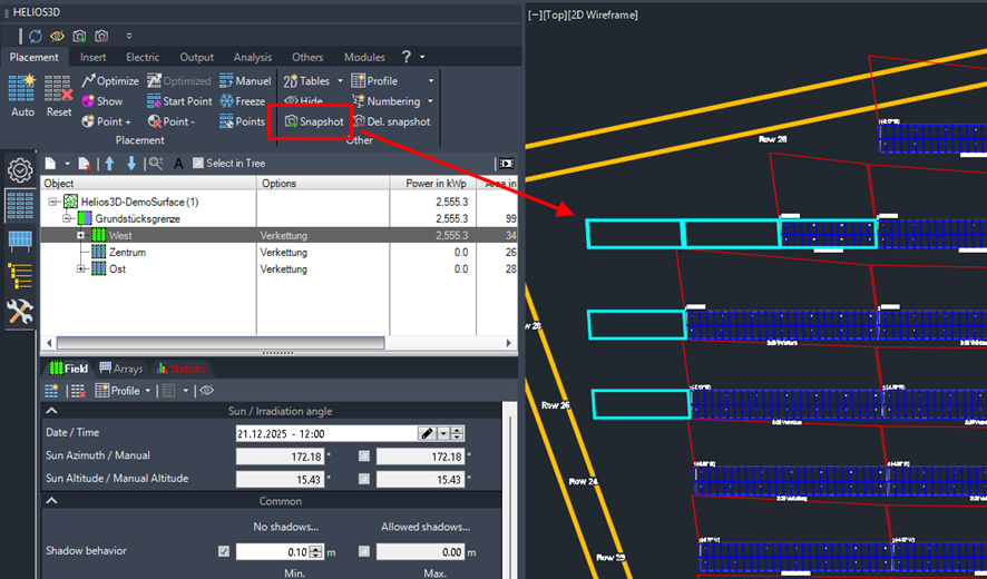
The placement page of the ribbon now also contains buttons to create snapshots or clear the target layer “H3D_Snapshot”. At the same time, now all available snapshot buttons work the same way and handle all available objects, so there is no need to create snapshots of electric elements by the electric page or temporary analysis markers by the corresponding menu. The new buttons, like the ones that existed before, can now be used to insert temporary markers for placement conflicts as in the next picture.
Snapshots are intended for temporary documentation, checking and communication. Snapshot objects are placed on the layer H3D_Snapshot and should not be confused with live Helios 3D placement objects. If the layout changes, create a new snapshot to document the updated state.
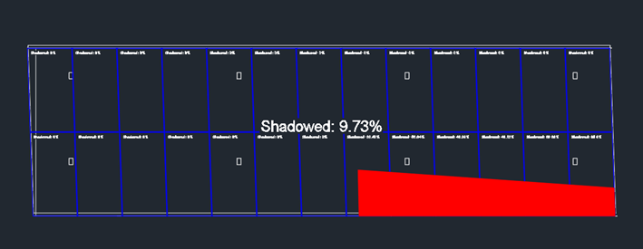
The shadows displayed on the modules by the function “Visualize Shadows on Modules” under Tools are also considered for snapshots now. The texts on the modules and the red shadow shape in the next picture will then be inserted as regular AutoCAD objects.
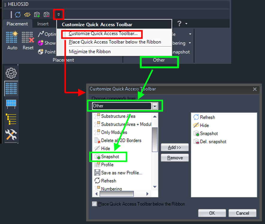
Users who use snapshots a lot might add the commands to the Quick Access Toolbar to avoid switching the tab page too many times.
Commands can be found by their command group and not by the tab page they are located on. The below picture shows the command group “Other” on the page “Placement” that contains the new snapshot command.
Deletes all objects on the snapshot layer
Deletes all objects found on the layer „H3D_Snapshot“.
Use this command only when the temporary snapshot objects are no longer needed. The command removes objects on the snapshot layer, but it should not be used as a method for changing the actual placement. Before deleting the snapshot layer content, make sure that the snapshot is not required for documentation, review or comparison.